Still inspired by binary subdivision trees

Introduction

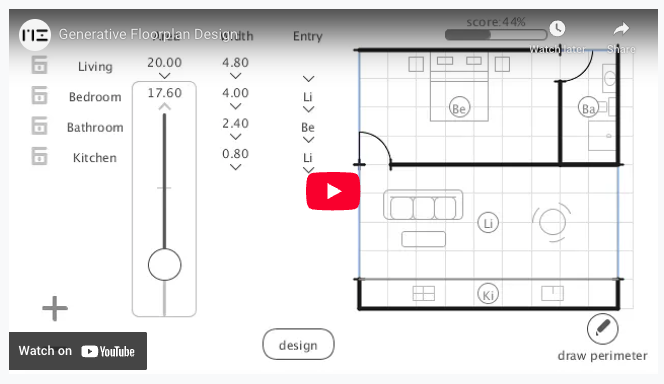
Binary subdivision trees (BST) as they apply to floor plans have probably been around for a while. The first time I saw them in the wild was probably when I came across my friend Martin Stacey’s thesis. The thesis uses a genetic algorithm (GA) to approximate a floor plan dataset. In other words there’s a database that includes various floorplans from which statistical metrics are derived. Then the GA is trained to yield a floorplan with a target set of rooms, while complying with allowed dimensional ranges and adjacency requirements. BSTs are essentially the geometry engine to create these floorplans. A few interesting components there which we will touch on later in the post. For now, check out a video of a demo application Martin built which is pretty cool:

By Martin Stacey

This blog post is mainly about getting acquainted with binary subdivision trees (BSTs, not to be confused with binary search trees), as well as reflecting on their qualities and their limitations for floor plan generation.

Disclaimer

Why get acquainted with BSTs, haven’t we moved past that?

State of the art floor plan generation has moved past using BSTs as the geometry engine for the model being optimized. While powerful they remain somewhat limited in what they can represent. But here’s a few reasons why I am choosing to do so:

• it might inspire interesting reincarnations of an old technique (when Martin has time to revisit)
• it’s a good excuse for me to build a minimal 2D geometry/topology library for representing spaces and their connectivity (which the world doesn’t need, but relates to the next point)
• it allows me to reboot my design/computation brain - the last couple of years I’ve been doing full stack web development first and foremost

BSTs

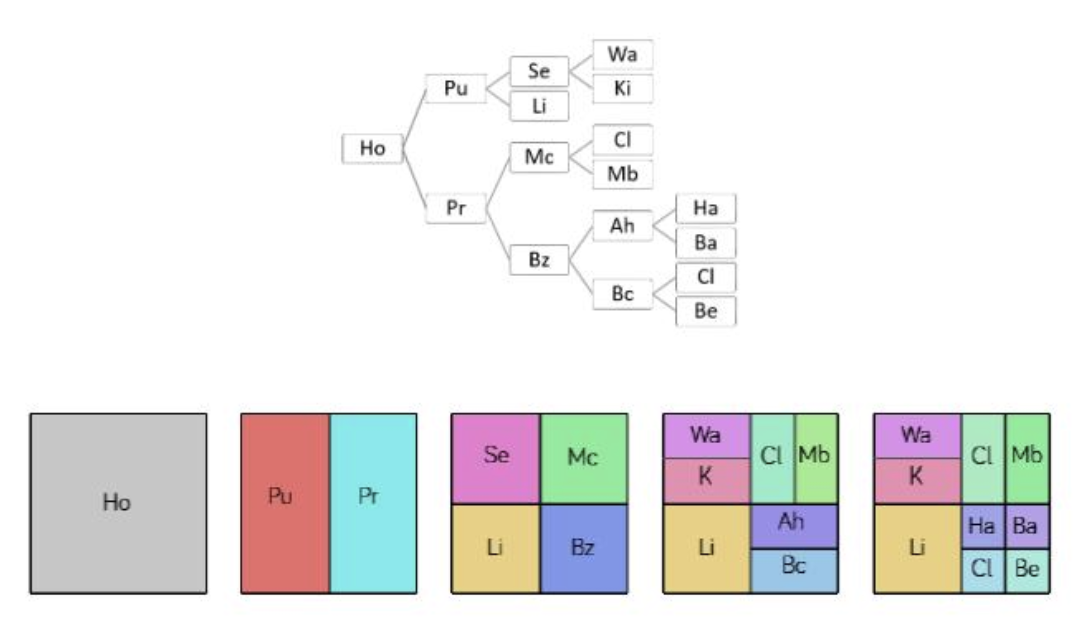
The image below illustrates what a BST is. It’s a tree so you have a root node, and then all other nodes which are either branches or leaves. The binary constraint means each node has either two children or none. Having a single child for BST implies a second child, even if that leaf is unassigned. My general intuition was that BSTs have some limitations in terms of the topologies they are able to represent. On page 25 Martin’s thesis cites the topological explorations of Steadman and Mitchels (in the 1970s) and claims that theoretically all floor plans can be represented by BSTs (with the exception of spiral configurations). I won’t be the one to disprove that given the amount of permutations possible.

By Martin Stacey

Topologies

Topology in this case refers to the tree’s signature; in other words what nodes are connected and at what levels, determining the arrangement of the tree. Handily, for any n number of leaves, we can use Catalan Numbers to determine the number of topologies for that leaf count.

The Catalan number formula is defined as:

This means the number of topologies alone grow (sub)exponentially. This doesn’t even account for the additional number of permutations (vertical / horizontal subdivision variants), which also grows exponentially. Find below a simple interactive component showcasing the space of available topologies for trees with 6 leaves. It is a truncated set, as I chose to remove topologies that are unbalanced (by 2 levels or more). But a true untruncated set for topologies with 6 leaves as provided by Catalan Numbers has a size of 132.

Topology Explorer

Permutations

When you actually consider the permutations possible given the horizontal or vertical subdivision at each branch, that number grows from Catalan Number to:

The total set for all permutations (horizontal & vertical subdivisions) with a leaf count of 6 is 8448. The component below represents that set (but again - truncated to be balanced by to 2 levels or less). Notice the legend: blue represents horizontal subdivisions, red represents vertical subdivisions.

Permutation Explorer

Set Sizes

To drive the point home, below is a table showing the set sizes for different arrangements:

• 2nd: all topologies
• 3rd column: all permutations
• 4th column: truncated topologies 2 levels difference or less
• 5th column: truncated permutations, 2 levels difference or less
• 6th column: truncated permutations, 1 level difference or less

As you can see the more balanced we require the trees to be (less difference between levels), the more we truncate the set of possible trees. There is probably a middle ground, however: if you truncate it too much then maybe you constrain the permutations available too much, too little and you end up with a giant set of unbalanced options that are likely not useful.

Notice that some cells haven’t been filled out. This is because my tree-generating algorithm crashed out when attempting to generate all truncated trees of a certain leaf count at that point. Different (more efficient) implementations might yield different results. There may be a formula that calculates the set size for all possible permutations given a certain level of balancing (balanced-1, balanced-2, etc). However I am not familiar with one, so I relied on my tree-generating implementation to give me a final count for those columns.

function* generateAllTrees(
  leaves: number,
  maxBranchDiff: number = 2,
): Generator<string> {
  if (leaves === 1) {
    yield 'L';
    return;
  }

  for (
    let leftLeaves = 1;
    leftLeaves < leaves;
    leftLeaves++
  ) {
    const rightLeaves = leaves - leftLeaves;

    const unbalanced =
      Math.abs(leftLeaves - rightLeaves) > maxBranchDiff;
    if (unbalanced) {
      continue;
    }

    for (const leftTree of generateAllTrees(
      leftLeaves,
      maxBranchDiff,
    )) {
      for (const rightTree of generateAllTrees(
        rightLeaves,
        maxBranchDiff,
      )) {
        yield `IV(${leftTree},${rightTree})`;
        yield `IH(${leftTree},${rightTree})`;
      }
    }
  }
}

Interactive BST!

Putting it all together: find below an interactive component to explore topologies and permutations and their resulting floorplan representation. To search through the design space, change the leaf count and the layout variation slider within the Topology tab. Then the Subdivision tab allows you to explore different subdivision values for the permutation in question. Clicking Animate lerps through a clamped range of subdivision values for the whole tree at once, for the permutation in question.

The colors of the resulting spaces correspond to their level on the tree. For a refresher on levels, have another look at Topology Explorer. Also notice the black dots at the center of each space, and the lines connecting them. This is the graph I mentioned in the introduction. Interestingly if you watch the animation (you need to trigger it from the Subdivison tab) you’ll see that some nodes become disconnected for certain lerp ranges. This seems to somewhat confirm Martin’s assertion that all (many) topologies are actually possible within the BST, if you lerp hard enough.

MVFS

There are probably many ways to go about building a floor plan solver. But if we had to express a Minimum Viable Floorplan Solver (MVFS), these are some inputs you might need at a minimum:

Constraints:

• Spaces: dimensions (min/max)
• Spaces: adjacencies (required/disallowed)
• Boundary: geometry

Of course depending on the typology (clinic, office, single family home, etc), you might have many other hard constraints including but not limited to min/max travel distances, min/max stair separations, etc. But if we stick to the innocent MVFS, we already have a few pieces to work with. The above constraints and maybe other objectives can lead to a series of fitness functions that help decide whether a solution is good or bad. To contextualize, BSTs occupy both the Topological Engine and Geometry Engine in the diagram below:

    
flowchart TD
  MVFS[MVFS] --> TE[Topology Engine]
  MVFS[MVFS] --> GE[Geometry Engine]
  MVFS[MVFS] --> C[Constraints]
  C --> FF[Fitness Function]
  MVFS --> OO[Other Objectives]
  OO --> FF

  

In a sense there we have all the pieces we need to build a MVFS. We can swap out different implementations for each of the above, refine the algorithms used for each of the pieces and so on.

The above approach assumes a solver of a stochastic optimization algorithm sort (GA or MOGA), generally known in AEC as Generative Design (GD).

What these algorithms do at a high level is search through a high dimensional design space using a degree of randomness. This approach is iterative, non deterministic, and can be pretty sensitive to parameters. It is not guaranteed to produce ‘good’ solutions. In the MOGA case the power is visualizing Pareto solutions across multiple objectives, and understanding the tradeoffs of some solutions versus others.

Limitations

BSTs are nice because they are elegant. Some limitations I see when you combine BSTs (as the geometric engine to solving floor plans) with a stochastic optimization approach:

• GA: You need to know the parameter count ahead of time, which requires retraining: see second point.
• GA: You aren’t pretraining the model, so the user basically has to wait for the training to happen. You can parallelize GA / MOGAs but still, you have to retrain it on the fly.
• GA & BST: You are spending a lot of time searching for: (1) the right topology (2) the right dimensions. If you have an adjacency table and allowable room dims, there are likely (?) more direct ways to translate that into a floor plan.
• GA: Performance degradation linear or worse as the size of the problem increases, which is not the case for other (especially pretrained) approaches.
• BST: A BST can only be fully evaluated once you draw out the entire thing, there is no partial evaluation and no ability for that reason to pair it with a backtracking algorithm.

Maybe a partial solution to the second point would be cutting out one of the searches (say the topology search) by storing the embeddings of all possible binary topologies in a database. That way, the stochastic optimization would only be in charge of fine-tuning where the binary divisions occur: ie getting the room dimensions right. Notice that the current algorithm can only deal with rectangles as a boundary geometry. One way around this is to decompose a more complex polygon into rectangles, and then break it into multiple GA subproblems. The approach presented by GPLAN in the Solve in real time section cuts through both of those: it presents techniques to convert a graph to a series of spaces, and it also addresses non-rectangular boundaries by breaking them into rectangles and solving for each.

Beyond GAs

As I understand it some of the floor plan optimization approaches fall into the following categories, there’s probably so many more.

Pretrained model inference

By frontloading the core problem solving (training and fine-tuning) during inference the model can be really fast.

Examples: This is exemplified by LLM foundation models. Google, Autodesk, and others in AEC are working to build these. Some datasets I have come across for this that could likely contribute to this approach are RPLAN and Swiss Apartments Dataset. Also, Jeroen from PlanFinder’s post suggests that OpenAI’s models is gaining capabilitiy in this space. One really exciting example in this space is the work shown in Reza Kakooee’s blog post series following his thesis.

Constraints: In the foundation model approach, I’m guessing the quality and diversity of your data matters a lot. For the RL approach, the barrier to entry to understand RL is probably the main constraint 😂.

Solve in real time

This includes classic GD, but also backtracking algorithms (think pathfinding algorithms for instance). By parallelizing where possible and offloading heavy computation to different processes you keep the UI responsive and your user engaged while results start landing.

Examples:(GA/MOGA/Backtracking algorithms). Most GD implementations or other solver implementations you’ve seen. To list a few in no particular order: Higharc, Finch3d, TestFit, among others. The difficulty here is that the line between a solver just procedural modeling can be sort of a thin one, especially if you don’t have access to the source code.

Constraints: Parameters, Hyperparameters, understanding the search space and ensuring diversity of solutions presented. Performance degrades linearly or worse with the problem size.

GPLAN

One sub-implementation that seems to be in its own category because of its determinism and performance, is the graph theoretical approach exemplified by GPLAN. I have yet to really understand the different pieces of their solver, but it seems to sidestep probabilistic solving (GA-like) with a more deterministic, mathematical approach.

Generally other ways to side-step heavy optimization is to break it down into smaller problems. We did this back at Outer Labs with some tools that would solve for ‘regions’ of the floorplans, or even just a room at a time. This makes the ‘solve-in-real-time’ tractable: the solver would put out a range of valid solutions without too much trouble given the size of the problem to solve.

Conclusion

Excited to see this space evolve! Maybe resolving floorplans algorithmically isn’t the most pressing problem of our time, but I think it still serves as a really interesting test bed for algorithm development.